If you want to study how standard costing works in a real manufacturing environment, you need data. Not a textbook table with three rows and two products — real data. Journal entries that trace material from purchase to WIP to finished goods. Labor records that capture skill-based rate differences across shifts. Overhead allocations that flow through departments before landing on products.
There are three ways to get this data. Each one has a problem.
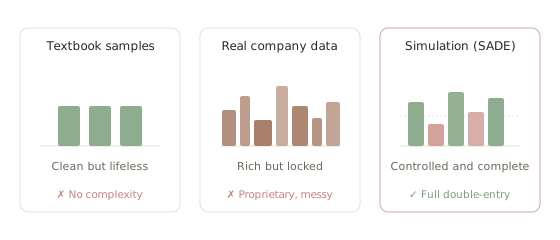
Textbook samples give you three products, two materials, and a neat variance table. You can verify the formula works. You learn nothing about what happens when a batch runs over capacity, when a supplier changes price mid-month, or when a trainee takes twice as long as a skilled operator on the same work center.
Real company data has all of that complexity — but you can’t get it. Manufacturing GL data is proprietary. Even anonymized, companies won’t share their cost structures. And if you do get access through an employer, the data is shaped by that company’s specific chart of accounts, ERP quirks, and allocation rules. It’s one example pretending to be general.
Simulation is the third path. You define the manufacturing process — bill of materials, routing, work centers, skill levels — and let the engine generate transactions day by day. Every purchase, every labor booking, every overhead allocation produces a balanced journal entry. The data is realistic because the model encodes real constraints: materials have waste rates, workers have skill-dependent speed factors, overhead follows a defined absorption methodology.
That’s why I built SADE. Not because simulation is elegant in the abstract, but because the question I wanted to answer — how do standard costing variances actually behave across a full production cycle? — couldn’t be answered with the data that was available to me.
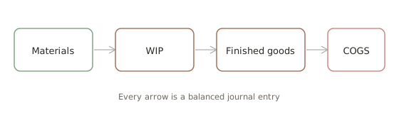
The engine runs for any number of days. Each day, it processes purchase orders, schedules production batches, books labor by worker and work center, absorbs overhead at predetermined rates, and transfers completed units. At period end, it calculates variances — material price, material usage, labor rate, labor efficiency, overhead volume, overhead expenditure — and posts them to the correct GL accounts.
The result is a complete, balanced set of financial records for a manufacturing company that doesn’t exist but behaves like one that does. That’s the dataset VIP will analyze.